Normal approximation for number of wins over a season

This blog post is regarding the discussion here. The question asked in the OP was if there was a good way to calculate the probability function for the number of total wins over a football season given the probability of winning the individual games. I had suggested that a normal approximation might be appropriate. However, there are some problems with using a normal approximation. Namely, the normal distribution is defined over the entire real number line and is symmetric about its mean. If E[X], where X a random variable used to describe the total number of wins over a season, was approximately 0 then a significant portion of our normal  distribution would be for X<0, which is obviously meaningless. I got curious to see how well a normal approximation would work given somewhat realistic probabilities, which is the subject of this post.

The true distribution that I should compare my normal approximation to is a Poisson binomial distribution, however calculating specific probabilities for that is a bit unwieldy. Therefore, instead of comparing my normal approximation to the true distribution, what I have done is written a piece of code using random trials to generate my distribution for me. I have then compared my normal approximation to my computer generated distribution.

Before delving into the details of my computerized experiment and analyzing how well a normal approximation reproduces its results some background on a normal distribution seems appropriate. According to the central limit theorem you can approximate the probability distribution for a function that is the sum of other random variables, each random variable subject to its own probability distribution function, as long as some basic conditions are met. In our case the result of each game can be represented as an independent random variable which takes a value of 1 for a win and 0 for a loss. The total number of wins for the season is then the sum of these random variables, and the central limit theorem should apply as long as the expected total number of wins isn’t too close to 0.

Based on the above paragraph, lets look at how to find a normal approximation. The normal distribution function is given by

where is the expected value and $\latex \sigma$ is the standard deviation. Since we’re looking for the distribution of a sum of random variables we can find the expected value and variance quite simply based on the individual random variables that are summed. Since the individual random variables can only be 1 or 0, if is the probability of winning the ith game then

.

Since we’ve assumed that we know the probability of winning each individual game it is straightforward to calculate the expectation value and standard deviation of our total distribution. Since this is all we need to know for a normal distribution, our normal distribution is therefore calculated. One final not about the normal approximation: note that the true probability distribution and my simulated probability distribution will be discrete, whereas a normal distribution is continuous. Therefore, to extract the chance of winning n games from the normal distribution I will use

where f(x) is the normal distribution function.

We now get to the heart of this post: my simulation and comparison with the normal approximation. I have simply picked fifteen different probabilities which represent the win probability. I have deliberately chosen them to be somewhat low, so we can see how much of the distribution is below zero, however they’re not too low so that they remain realistic as all of the teams in question are, after all, in the same league. The probabilities I’ve used for winning are {0.1, 0.2, 0.3, 0.3, 0.1, 0.1, 0.2, 0.3, 0.2, 0.3, 0.1, 0.5, 0.1, 0.2, 0.2}. These should be about what the Aggie football team’s winning chances will be next year per game (I’m just kidding, don’t lynch me!). Based on these probabilities we can expect this team to win 3.1 games next year with a standard deviation of 1.51.

My code, which is given below, is structured so that the trials loop simulates an entire season. The wins variable stores the total number of wins for the season, and is initialized to zero. The game loop simulates each game with a random variable. The random variable takes a value between 0 and 99. If the value is less than the probability of winning that game multiplied by 100 then the game counts as a win and the wins variable is incremented. After all the games are simulated, the element of the totalwins array corresponding to the particular number of wins in the season is incremented. After a million simulated seasons, I print out the totalwins array divided by 1000000, which gives us our simulated probability distribution.

The code for my simulation is given below:

#include <stdio.h>
#include <stdlib.h>
#include <time.h>

int main(void)
{
	int totalwins[16];
	srand((unsigned)time(NULL));
	double probabilities[] = {0.1, 0.2, 0.3, 0.3, 0.1, 0.1, 0.2, 0.3, 0.2, 0.3, 0.1, 0.5, 0.1, 0.2, 0.2};
	int trial;

	// initialize total wins array
	int i;
	for(i=0; i<16; i++)
	{
		totalwins[i]=0;
	}

	for(trial = 0; trial<1000000; trial++)
	{
		int game;
		int wins = 0;
		for(game=0; game<15; game++)
		{
			int r = rand() % 100;
			if(r < probabilities[game]*100)
			{
				wins++;
			}
		}
		totalwins[wins]++;
	}
	
	for(i=0; i<16; i++)
	{
		printf("%f\n", (double)totalwins[i]/1000000);
	}
	
	return 0;		
}

Finally, lets examine how well our normal approximation reproduces our simulated results. A graphical and tabular representation of the data is given below.

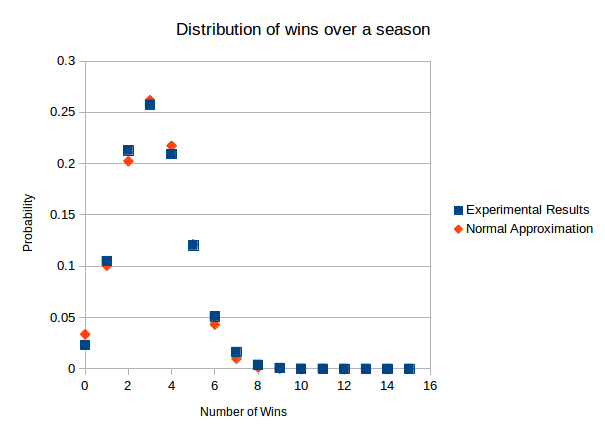
Wins	Experimental Results	Normal Approximation
0	0.023104	0.0336
1	0.104996	0.1005
2	0.21288	0.2023
3	0.257459	0.2618
4	0.209222	0.2174
5	0.120272	0.1214
6	0.05099	0.0432
7	0.016359	0.0099
8	0.003874	0.0015
9	0.000749	0.0001
10	0.000091	0
11	0.000004	0
12	0	0
13	0	0
14	0	0
15	0	0

One quick note about the tabulated data. Obviously none of the values are truly zero for the normal approximation. However, the values were so low for wins > 9 that my calculator could not distinguish them from zero.

Based on the graphical representation of the data, it should be clear that the normal approximation is indeed a reasonable approximation of the probability distribution. I think a few quick notes about some of the quantitative characteristics of the data are in order. First of all, less than 2% of the normal distribution lies below zero. It seems that our concern about the probability distribution being skewed that was is mostly unfounded. Secondly, the largest discrepancy between the simulated number of wins and the normally approximated number of wins is 1.3% for zero wins. The rest of the percentages are reasonably close. Finally, the correlation between the two data sets is .998. I want to point out that I only used two significant figures for my standard deviation. I suspect that the match between the simulated and approximated data sets would be even better if I used a more precise standard deviation.

Based on this, we can conclude the following. If you need exact results, calculate the Poisson binomial distribution function recursively as indicated in section 2 of this paper. However, only do this if you need exact results, as the calculations are a bit unwieldy. You could instead come up with a simulated probability distribution as I have done in my code. However, if you would prefer to work analytically and you don’t need exact results, based on my above analysis it seems perfectly valid to use a normal approximation. The normal approximation should give you reasonable results.