Why Flat Spacetime is Infinite

April 7, 2016April 7, 2016 dargscisyhp

In the Texags post Arguments for and Against the Existence of God Letters at Random asked why a flat space is infinite. I thought this would make a good topic for a post on this blog. I will first discuss a little bit about the relativistic concept known as proper distance. Next, we will briefly discuss the metric and how it relates to curvature. Once these concepts are discussed I will finally introduce the FLRW metric, the mathematical equation that governs the structure of our universe on the large scale, and show why a flat spacetime will be infinite.

The concept of measurement in relativity is a bit more complicated than in regular classical mechanics. The reason for this is that in classical mechanics there is a universal clock, and all things can be measured simultaneously. However, in relativity the simultaneity of two events depends on the reference frame of the observer. Therefore things like the length of an object and the elapsed time between two events also depends on the observer. All of this is true in special relativity.

When the curvature of general relativity is added to the mix things get even hairier. Time and length measurements now also depend on the path you are taking through spacetime. Because of this any length or time measurement you make in curved spacetime can only be local. So how do we deal with this? Well, we use what the geometry of spacetime gives us. We use a concept known as proper distance.

To get an idea of what proper distance is, let’s discuss its analogue in ordinary Euclidean space first. If I ask you where an object is located you can simply tell me its coordinates. You might say one endpoint is at (0,0) and the other endpoint is at (3,4). If I asked someone else with an origin two units behind the first observer they will tell me the endpoints are at (-2,0) and (1,4). If I asked someone else whose coordinate frame was rotated with respect to the first two coordinate frames they might tell me the endpoints are at (-1,0) and (4,0). These would all describe the same object, but they don’t really give us any information about the object itself, they tell us at least as much about the location and orientation of an observer’s origin. If we wanted to truly learn something about the object we would want something that does not depend on the location and orientation of an observer’s origin. In physicist lingo, we want a measure of the object that is translationally and rotationally invariant. Thankfully, today even school children are equipped with the Pythagorean theorem and they could easily tell you that the length of the object is five units. Length is the ordinary analogue of relativistic proper distance. In Euclidean space, the infinitesimal length, or metric in physics terminology, is given by

$ds^2=dx^2+dy^2.$

This might be a little different than the Pythagorean theorem you’re used to seeing, but it’s essentially just the infinitesimal version of it. As an aside, this is precisely why you can’t view Euclidean space as three simple one dimensional spaces haphazardly stiched up. A truly frame-indepdent, geometric quantity about an object is based on its existence in two dimensions simultaneously (or three or however many dimensions you’re working in). A string of one-dimensional numbers means nothing about the object until you combine them appropriately.

The metric can do more than just give us the line element in flat space, though. It can also handle curved spaces. For instance, the metric on the surface of a sphere is

$ds^2=dr^2+r^2 d \theta^2+ r^2 \sin^2 \theta\ d \phi^2.$

The details of this metric aren’t important, but it might be of interest to understand conceptually how this comes about. Basically what you do is locally consider the space flat (think about the Earth — locally it is basically flat), apply the flat-space metric and get an infinitesimal line element, keep moving along the path that you’re taking and stringing up the infinitesimals that you get using calculus. Working through all the mathematical details will get you a metric like above. If you look at the metric the coefficients in front of the infinitesimals are scaling factors to account for your curvature.

Now, let’s enter the realm of spacetime. The metric of an isotropic, homogeneous universe is given by

$ds^2= -dt^2 + a^2(t) \left[ \frac{dr^2}{1 - kr^2} + r^2 d \Omega^2 \right]$ .

There is plenty of experimental evidence that on the large scale the universe is both homogeneous and isotropic, so this metric is appropriate. The derivation of this metric is beyond the scope of this post, but it’s basically the same thing as what we’ve done above, just describing a different geometry. Here t is the local time variable, r the radial variable, omegna the angular variable, a is a scaling factor which describes the expansion of the universe, and k is the curvature of the universe. If k takes a value greater than 0 then we have a closed universe, if it is less than 0 then we have an open universe, and if it’s 0 then we have a flat universe. You can read more about the shape of the universe here. We can set a(t) to 1 without losing anything from this discussion. Furthermore, we can only vary the radial coordinate to simplify the discussion mathematically and see what happens. In that case, the metric becomes

$ds^2 = \frac{dr^2}{1 - kr^2}.$

This is satisfied by the following path:

$s(r) = \frac{\sin^{-1}(\sqrt{k}r)}{\sqrt{k}}.$

The proper distance is maximized when the argument of the arcsin is 1, or when $r=k^{-1/2}$ . Thus the maximum proper distance is

$\frac{\pi}{2 \sqrt{k}}$

It’s straightforward to see that as k goes to 0 the maximum proper distance goes to infinity. This is what is meant when people say a flat universe is infinite. There is also some evidence indicating that the universe is indeed flat.

Addendum for the physics buffs: I have treated the universe as simply connected here to avoid discussing any weird topologies.

Please direct all discussion to the associated Texags post.

Will a Plane in Straight and Level Flight “Ascend” Away from the Curvature of the Earth?

February 3, 2016February 3, 2016 dargscisyhp

On the Texags Politics thread on flat Earthers there was some disagreement about why a plane does not ascend away from the curvature of the Earth. I commented that to understand why a plane doesn’t ascend away from the Earth in straight and level flight we have to realize how big the Earth is. I clarified this comment by stating that for every mile of flight the Earth descends about eight inches, and that this descent is accounted for by the microcorrections made during flight. KeithDB suggested that “the plane flies at a max altitude and thus stays with a certain limit above the sphere, traveling in an arc around the sphere as it goes.” ’03ag stated that “through air speed or manipulating control surfaces you can generate an amount of lift equal to the force of gravity. Once those settings are found you will fly at a constant altitude. they don’t need to change unless atmospheric conditions change.” He further stated that since lift and gravity cancel each other out giving you a net zero radial force component, “your distance to the center of this radial force remains constant.” He seemed to disagree with me when I stated that the form of Newton’s second law had to be changed in order to account for curvilinear polar coordinates. Finally, JJxvi stated that “In a perfectly stable atmosphere, I believe the pilot could set his controls where lift=gravity and the plane would automatically fly in a orbit pattern just as something orbits the earth without needing course correction.”

Obviously there is considerable disagreement between myself and others on the politics board regarding why a plane does not naturally ascend. It is my goal in this post to show that the true explanation of why a plane does not naturally ascend is a bit more subtle than what is being suggested by others. Namely, I aim to show that setting lift force equal to the gravitational force does not produce a circular path. In fact, it produces a path in which the plane ascends if it is initially flying parallel to the ground. I then wish to look at a situation which may not yet have been mentioned (it has been explicitly mentioned since I began writing this post): the case that the lift force is just less than the gravitational force so that the combination of those two forces gives us a force consistent with a true net centripetal force. I argue that this explanation is implausible. Finally I look at the case where the plane must correct its flight path. I show why the size of the Earth matters, and how it obscures the necessary corrections.

We begin with some math that will be necessary to explore this phenomenon in greater detail. First of all, we will only consider direct flights between two points on the globe. This simplifies the mathematics so that everything can be examined in two dimensions. The relevant information we need is the plane’s height above the ground and how far it is into its trip. For the purpose of this post I will use two different representations for this information. I will use the typical Cartesian coordinates and I will use polar coordinates, with the center of the Earth as the origin in both instances. In Cartesian coordinates we can write the position vector as

$\vec{R}=x \hat{x} + y \hat{y}.$

The height of the plane can be extracted from here as follows:

$h=\sqrt{x^2+y^2}-r_e,$

where $r_e$ is the radius of the Earth. On the other hand, we can write the position vector in polar coordinates as

$\vec{R}=r \hat{r},$

here r is the radial distance of the plane from the center of the Earth. Height is then simply $h=r-r_e.$ We need a second coordinate in polar coordinates. That will be the angular displacement. So in polar coordinates we have r for the height and $\theta$ for the angular displacement. We can relate the Cartesian and polar representations as follows:

$x=r \cos \theta$

$y=r \sin \theta$

$r= \sqrt{x^2+y^2}$

$\hat{r}=\cos \theta \hat{x} + \sin \theta \hat{y}$

$\hat{\theta} = - \sin \theta \hat{x} + \cos \theta \hat{y}.$

We now come to the physics. The only relevant physics we need to know is Newton’s second law: $\vec{F}=m\ddot{\vec{R}},$ and what forces are relevant. In its vector format Newton’s second law is equally valid in Cartesian and polar coordinates. If we look at Newton’s second law in a particular Cartesian component, its form will not change:

$\dot{\vec{R}}=\dot{x}\hat{x}+\dot{y}\hat{y},$

$\ddot{\vec{R}}=\ddot{x}\hat{x}+\ddot{y}\hat{y}.$

$\vec{F}=m\ddot{\vec{R}}=m(\ddot{x}\hat{x}+\ddot{y}\hat{y})=ma_x \hat{x}+ma_y \hat{y}$

However, the form of Newton’s second law changes for a polar component since the coordinate system itself varies with time. In that case we have

$\dot{\vec{R}}=\frac{d}{dt} \left[ r \hat{r} \right] =\dot{r} \hat{r} + r \dot{\hat{r}},$

$\dot{\hat{r}} = \frac{d \hat{r}}{d \theta} \frac{d \theta}{dt} = \hat{\theta} \dot{\theta},$

$\dot{\vec{R}}=\dot{r} \hat{r} + r\dot{\theta} \hat{\theta}.$

The second derivative can be found simply by taking the derivative of the above expression, where to get the time derivatives of the polar unit vectors we go back to their definition and use the chain rule. The second derivative is

$\ddot{\vec{R}} = \left( \ddot{r} - r \dot{\theta}^2 \right)\hat{r} + \left( 2 \dot{r} \dot{\theta} + r \ddot{\theta} \right) \hat{\theta}.$

Therefore, Newton’s second law in polar components is

$F=m \ddot{\vec{R}} = m \left( \ddot{r} - r \dot{\theta}^2 \right)\hat{r} + m \left( 2 \dot{r} \dot{\theta} + r \ddot{\theta} \right) \hat{\theta}.$

Obviously the form of Newton’s second law is not preserved in polar components, because if it was the above equation would be

$F=m \ddot{\vec{R}} = m \ddot{r} \hat{r} + m \ddot{\theta} \hat{\theta}.$

One final thing to note about the polar formalism was that it was derived very generally. We did not assume anything to be moving in a circle. However, we can see where the introductory physics centripetal acceleration formula comes from in the above equation. Obviously, for the radius to remain unchanged it is necessary that the radial component of the force is directed inward with a magnitude

$r \dot{\theta}^2=\frac{v^2}{r}.$

The final piece of physical information we want to consider before examining particular scenarios is what forces we will be looking at. At any instant in time let’s break all the forces into components that are perpendicular or parallel to the ground. To make this problem a little simpler, we will assume that the plane is going at a constant speed parallel to the ground. This means we only have to worry about physics in the dimension perpendicular to the ground. In that dimension, we will have gravity, which will be denoted by $F_g$ , and lift, which will be denoted by $F_l.$ Gravity is simple. Newton told us that gravity is

$F= -\frac{Gm_em}{r^2} \hat{r},$

where $m_e$ is the mass of the Earth and m is the mass of the plane, as before, and the minus sign denotes that gravity pulls towards the Earth rather than pushes away. The physics of lift, on the other hand, is far more complicated. You have to worry about atmospheric conditions, the geometry of the wing, the attack vector etc. Luckily for us, we won’t have to worry about any of that as the lift will be completely determined by the situation that we are analyzing, as we will soon see.

Now that we have the math and underlying physics down, let’s look at our relevant examples. First, let’s examine what happens when $F_l=F_g,$ or in other words when lift perfectly balances out the force of gravity. In this case, the net force on our plane is zero. So what happens to a plane if it’s flying parallel to the ground? We can position the plane so that in Cartesian coordinates it is initially at (0, y), and therefore will have a height of $h_i=y-r_e$ . After flying for an infinitesimal amount of time it will be at (dx, y) in that same cartesian coordinate system, and its new height, $h_0$ will be

$(h_0=\sqrt{dx^2+y^2}-r_e) > (\sqrt{y^2}-r_e=y-r_e=h_i)$ ,

$h_0>h_i.$

As we can see, the plane does indeed ascend when it is flying parallel to the ground and the lift force is equal and opposite of gravity. The reason I’ve done the above analysis for an infinitesimal translation is to account for the possibility that for a physical translation gravity and/or lift may change by an appreciable amount even in our hypothetical situation where the atmosphere is spherically symmetric. However, if we plug in realistic numbers such as dx=10 km and initial height at 8km then:

$h_0=\sqrt{10^2+6379^2}-6371=8.007$

or in other words, after flying ten kilometers the plane should have ascended seven meters. An ascent of seven meters will not change gravity or lift appreciably. We can, for all intents and purposes, say that over that flight of 10 kilometers the gravity and lift remain constant, and thus constantly cancel. So while my initial calculation was for an infinitesimal translation, we can see that this effect is real over 10 km when we plug in actual numbers, and weird things like varying gravity or varying lift can’t overcome this effective ascent in this case. So here, the ascent is real.

Before moving on, let’s examine this case in one other way. Recall that the radial component of Newton’s second law is

$F_r = m \left( \ddot{r}-r \dot{\theta}^2 \right).$

Since we’re examining the case where gravity is equal and opposite of lift, we have $F_r=0$ and

$\ddot{r}=r \dot{\theta}^2.$

Since, for the plane to fly, $\dot{\theta} \neq 0$ it is clear that the radius is increasing from the polar formalism as well. We can positively conclude from this discussion that if a plane is flying parallel to the ground and the lift force is equal and opposite of gravity, the plane will spontaneously “rise” in the sense that it will fly away from the curvature of the Earth. Obviously this ascent is limited in range as ultimately lift will decrease as the atmosphere thins out, but for a distance like 10km this is a real effect when flying parallel to the ground with your forces in equilibrium. At this point it should be amply demonstrated that in the case where we “have equivalent lift acting parallel and in the opposite direction” to gravity, the idea of a plane ascending is not “flatly wrong on paper and in practice,” as was suggested on the forums.

The next thing to examine is what happens when we have the “Goldilocks lift,” or when the lift is just right so that it counteracts gravity exactly to produce a net centripetal force:

$(F_g-F_l) \hat{r} = -\frac{mv^2}{r} \hat{r}.$

It is true that were this condition met then you would have a plane that travels in a circular path around the globe. But this probably isn’t exactly what’s going on either. To see why, we’ll have to look at the actual numbers.

On the forums it was suggested that by moving out of the idealized world of physics I’m moving the goalposts. This is not the case. The situation we were discussing when using the idealized physics model was the first one. The claim was made by several posters that in the idealized case that lift equals gravity the plane would fly in a circle around the globe. I have shown that’s not true. It’s an entirely different claim that if the Goldilocks lift were hit and maintained that the plane would fly in a circle around the globe in the idealized model. That claim is true in the idealized model. The Goldilocks lift is probably not maintainable throughout a flight in reality, though.

Essentially, on average, you’re probably right. Once the plane hits its cruising altitude its average lift probably is the Goldilocks lift. But I don’t think the airplane maintains its course by carefully measuring and regulating the lift force. The difference between the gravitational force and the lift force to hit the Goldilocks lift is about 0.1% of the total lift force. I know when I flew Cessna 172s there was absolutely no way I could regulate the lift that precisely. I doubt even state-of-the-art airplanes could regulate it to that precision. Even in the physically idealized perfectly spherically symmetric atmosphere, regulating your lift that precisely over the course of an entire flight would probably not be possible. As such, course corrections would have to be made to keep the plane at a stable altitude.

The reason that this argument might be seductive is that it is predicated on the assumption that planes fly parallel to the ground. This is how it looks to anyone who has piloted an aircraft or taken a flight on an aircraft. However, if you make that assumption, you end up with the first situation. Checkmate round-Earthers! But not so fast. If you aim the plane towards the horizon it flies very close to the Goldilocks lift. However, the difference in angle between aiming for the horizon and flying parallel to the ground is practically imperceptible. This is due to the enormity of the Earth relative to how high we fly above it (I can work the math out on this if anyone wants to see it). When the biggest reference point we see while flying is the ground and it appears to us that we are flying parallel to it, it’s natural to assume that that is indeed the case, and we are quickly lead to the first situation: we are flying parallel to the ground with lift being equal and opposite of gravity. The second factor in not noticing this effect must be the fact that the lift is not perfectly controllable, and as such the pilot or the autopilot is always making minor corrections to its course. Seeing that the Earth curves away from a plane flying parallel to the ground so slowly, again due to the enormity of the Earth, this effect must get lost in the noise of those corrections as the pilot or autopilot will indeed correct to fly at the correct.

So I hope I have convinced you of a few things. One, that in the case that the lift is equal to the gravitational force and the plane is flying parallel to the ground the plane will indeed ascend spontaneously. Two, since lift cannot be maintained at an absolute constant it is not correct to assume that setting the plane to the perfect level of lift is the ultimate answer to why planes fly in a circle around the globe. Corrections would still need to be made. Three, I hope I’ve shown why this argument is seductive, as it appeals to intuition about how planes fly and then it appeals to the first situation, where gravity and lift are equal and opposite. And finally, I hope I have shown that the seductive, intuitive argument is fallacious, and you can realize the fallacy by realizing just how enormous the Earth is.

Please direct all discussion regarding this post to the relevant Texags threads.

Normal approximation for number of wins over a season

January 8, 2016January 8, 2016 dargscisyhp

This blog post is regarding the discussion here. The question asked in the OP was if there was a good way to calculate the probability function for the number of total wins over a football season given the probability of winning the individual games. I had suggested that a normal approximation might be appropriate. However, there are some problems with using a normal approximation. Namely, the normal distribution is defined over the entire real number line and is symmetric about its mean. If E[X], where X a random variable used to describe the total number of wins over a season, was approximately 0 then a significant portion of our normal distribution would be for X<0, which is obviously meaningless. I got curious to see how well a normal approximation would work given somewhat realistic probabilities, which is the subject of this post.

The true distribution that I should compare my normal approximation to is a Poisson binomial distribution, however calculating specific probabilities for that is a bit unwieldy. Therefore, instead of comparing my normal approximation to the true distribution, what I have done is written a piece of code using random trials to generate my distribution for me. I have then compared my normal approximation to my computer generated distribution.

Before delving into the details of my computerized experiment and analyzing how well a normal approximation reproduces its results some background on a normal distribution seems appropriate. According to the central limit theorem you can approximate the probability distribution for a function that is the sum of other random variables, each random variable subject to its own probability distribution function, as long as some basic conditions are met. In our case the result of each game can be represented as an independent random variable which takes a value of 1 for a win and 0 for a loss. The total number of wins for the season is then the sum of these random variables, and the central limit theorem should apply as long as the expected total number of wins isn’t too close to 0.

Based on the above paragraph, lets look at how to find a normal approximation. The normal distribution function is given by

$f(x)=\frac{1}{\sigma \sqrt{2 \pi}}e^{-\frac{(x-\mu)^2}{2 \sigma^2}},$

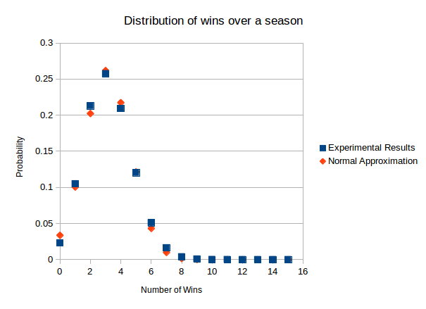
where $\mu$ is the expected value and $\latex \sigma$ is the standard deviation. Since we’re looking for the distribution of a sum of random variables we can find the expected value and variance quite simply based on the individual random variables that are summed. Since the individual random variables can only be 1 or 0, if $p_i$ is the probability of winning the ith game then

$\mu = \sum_i p_i$

$\sigma^2 = \sum_i (1-p_i)p_i$ .

Since we’ve assumed that we know the probability of winning each individual game it is straightforward to calculate the expectation value and standard deviation of our total distribution. Since this is all we need to know for a normal distribution, our normal distribution is therefore calculated. One final not about the normal approximation: note that the true probability distribution and my simulated probability distribution will be discrete, whereas a normal distribution is continuous. Therefore, to extract the chance of winning n games from the normal distribution I will use

$P[x=n]=\int_{n-0.5}^{n+0.5} f(x)dx$

where f(x) is the normal distribution function.

We now get to the heart of this post: my simulation and comparison with the normal approximation. I have simply picked fifteen different probabilities which represent the win probability. I have deliberately chosen them to be somewhat low, so we can see how much of the distribution is below zero, however they’re not too low so that they remain realistic as all of the teams in question are, after all, in the same league. The probabilities I’ve used for winning are {0.1, 0.2, 0.3, 0.3, 0.1, 0.1, 0.2, 0.3, 0.2, 0.3, 0.1, 0.5, 0.1, 0.2, 0.2}. These should be about what the Aggie football team’s winning chances will be next year per game (I’m just kidding, don’t lynch me!). Based on these probabilities we can expect this team to win 3.1 games next year with a standard deviation of 1.51.

My code, which is given below, is structured so that the trials loop simulates an entire season. The wins variable stores the total number of wins for the season, and is initialized to zero. The game loop simulates each game with a random variable. The random variable takes a value between 0 and 99. If the value is less than the probability of winning that game multiplied by 100 then the game counts as a win and the wins variable is incremented. After all the games are simulated, the element of the totalwins array corresponding to the particular number of wins in the season is incremented. After a million simulated seasons, I print out the totalwins array divided by 1000000, which gives us our simulated probability distribution.

The code for my simulation is given below:

#include <stdio.h>
#include <stdlib.h>
#include <time.h>

int main(void)
{
	int totalwins[16];
	srand((unsigned)time(NULL));
	double probabilities[] = {0.1, 0.2, 0.3, 0.3, 0.1, 0.1, 0.2, 0.3, 0.2, 0.3, 0.1, 0.5, 0.1, 0.2, 0.2};
	int trial;

	// initialize total wins array
	int i;
	for(i=0; i<16; i++)
	{
		totalwins[i]=0;
	}

	for(trial = 0; trial<1000000; trial++)
	{
		int game;
		int wins = 0;
		for(game=0; game<15; game++)
		{
			int r = rand() % 100;
			if(r < probabilities[game]*100)
			{
				wins++;
			}
		}
		totalwins[wins]++;
	}
	
	for(i=0; i<16; i++)
	{
		printf("%f\n", (double)totalwins[i]/1000000);
	}
	
	return 0;		
}

Finally, lets examine how well our normal approximation reproduces our simulated results. A graphical and tabular representation of the data is given below.
data

Wins	Experimental Results	Normal Approximation
0	0.023104	0.0336
1	0.104996	0.1005
2	0.21288	0.2023
3	0.257459	0.2618
4	0.209222	0.2174
5	0.120272	0.1214
6	0.05099	0.0432
7	0.016359	0.0099
8	0.003874	0.0015
9	0.000749	0.0001
10	0.000091	0
11	0.000004	0
12	0	0
13	0	0
14	0	0
15	0	0

One quick note about the tabulated data. Obviously none of the values are truly zero for the normal approximation. However, the values were so low for wins > 9 that my calculator could not distinguish them from zero.

Based on the graphical representation of the data, it should be clear that the normal approximation is indeed a reasonable approximation of the probability distribution. I think a few quick notes about some of the quantitative characteristics of the data are in order. First of all, less than 2% of the normal distribution lies below zero. It seems that our concern about the probability distribution being skewed that was is mostly unfounded. Secondly, the largest discrepancy between the simulated number of wins and the normally approximated number of wins is 1.3% for zero wins. The rest of the percentages are reasonably close. Finally, the correlation between the two data sets is .998. I want to point out that I only used two significant figures for my standard deviation. I suspect that the match between the simulated and approximated data sets would be even better if I used a more precise standard deviation.

Based on this, we can conclude the following. If you need exact results, calculate the Poisson binomial distribution function recursively as indicated in section 2 of this paper. However, only do this if you need exact results, as the calculations are a bit unwieldy. You could instead come up with a simulated probability distribution as I have done in my code. However, if you would prefer to work analytically and you don’t need exact results, based on my above analysis it seems perfectly valid to use a normal approximation. The normal approximation should give you reasonable results.

Ion Beam Notes

October 9, 2015 dargscisyhp

handout2

Renormalization notes

August 28, 2015 dargscisyhp

http://www.physics.umd.edu/courses/Phys851/Luty/notes/renorm.pdf

State Space of a Free Particle

July 27, 2015July 28, 2015 dargscisyhp

In the Texags R&P thread The Paradox of Creation I made a post stating that the state of a free electron is infinite dimensional. User Silent For Too Long asked me to elaborate to what I meant by that, which is what I intend on doing in this post. I will try not to go into the details of quantum mechanics beyond what is necessary to discuss the dimensionality of a free particle. I will begin by discussing a little bit about the Schrodinger equation in general. We will interpret the solution to the Schrodinger equation in the language of vector spaces. I will then apply the previous discussion to the free particle. Finally, I will try and motivate why we should discuss the free particle, and quantum mechanics in general, in that language.

The Schrodinger equation is central to all of quantum mechanics. It is a second order partial differential equation and is analogous to Newton’s F=ma in that it governs all dynamics on the quantum scale. It is

$i \hbar \frac{\partial \psi(\textbf{r},t)}{\partial t} = -\frac{\hbar^2}{2m} \nabla^2 \psi(\textbf{r}, t) + V(\textbf{r},t) \psi(\textbf{r},t).$

The only physical parameters that are important to our discussion are $\psi$ , called the wavefunction which is what we are solving for, and V, called the potential which is already known. Everything else can be thought of as constants. The potential contains all the information regarding the surroundings of the object that we’re studying, while the wavefunction contains all of the information regarding the object we’re studying itself. The usual process is we take the Schrodinger equation, plug in all the information that we have about our surroundings in V, and solve for the wavefunction. The way we extract useful physical information from the wavefunction is a little odd at first glance, but it doesn’t take long to get used to. Nevertheless, extracting physical information from the wavefunction is beyond the scope of this post. Here, we only aim to find it and discuss its dimensionality.

If the potential is not time-dependent then the Schrodinger equation can be solved through separation of variables. We can write $\psi = \phi(\textbf{r}) \chi(t).$ Without going through the gory details, this gives us

$\chi (t) = Ae^{-i \omega t} = Ae^{-iEt / \hbar}$

$-\frac{\hbar^2}{2m} \nabla^2 \phi +V \phi = E \phi$

The second of the above set of equations is called the time-independent Schrodinger equation. Here, the constant that the separated equations are set to are $\hbar \omega = E$ where $\omega$ is called the angular frequency and E is called the energy. The solution to the above for a particular value of E is called a stationary state and is given by

$\psi(\textbf{r}, t) = \phi(\textbf{r}) e^{-iEt/ \hbar}.$

These are called stationary states because the time evolution of the state (wavefunction) is just a phase-shift in the complex plane. Phase shifts of solutions to the time-independent Schrodinger equation don’t change any of the physical information contained in them, thus the evolution of such a state is said to be stationary. One of the important facts about stationary states is that they are orthogonal. Since the Schrodinger equation is linear, a superposition of orthogonal stationary states is also a solution to the Schrodinger equation (though it’s not necessarily a stationary state). Note to get the full solution of the Schrodinger equation you have to superpose all stationary states for all values of energy. We can look at the space spanned by all such stationary states. This space is known as the state space which is a Hilbert Space. The state of any quantum system can be thought to be a point in the state space located at the coordinate associated with the coefficients of the superposition. Now that we have discussed the Schrodinger equation and the state space a little bit we can apply it to the free particle, and look at its state space.

A free particle is one where there is no surrounding potential. In that case, we set V=0 in the Schrodinger equation. Without going through the details, the stationary states are

$\psi(\textbf{r},t) = Ae^{i \left[\textbf{k} \cdot \textbf{r} - \omega(k) t \right]},$

and using the superposition principle we see that the total wavefunction is

$\psi(\textbf{t},t) = \frac{1}{(2 \pi)^{3/2}} \int g(\textbf{k}) e^{i \left[\textbf{k} \cdot \textbf{r} - \omega(k) t \right]} d^3k$

Here the integral represents your summation, the g(k) represent your coefficients, and the rest of the integrand are your stationary states. Thus, you have represented your total wavefunction as a superposition of stationary states. What’s more, we can tell from the form of the integrand that any wavefunction can be expressed in that form given the right selection of g(k), since the integral is a Fourier transform. The integral runs over all values of k, thus we are summing together an infinite number of stationary states. Since we need an infinite number of stationary states to span the entire state space it is clear that the state is infinite dimensional. This is what I set out to demonstrate.

But we can ask one more following question: why even discuss this stuff in terms of state spaces. Why not simply call it a Fourier transform and leave it at that. Beyond the unsatisfying answer that all of this has the structure of (almost) a vector space and therefore we should examine it from that angle, there is another answer as well. The most general form of the Schrodinger equation is not the partial differential equation I gave above. It is

$i \hbar \frac{\partial}{\partial t}\Psi = \hat H \Psi$ .

This is an operator equation. Here H represents an operator and $\Psi$ represents a vector. Remember that vectors and operators are geometric objects that are independent of the basis you used to represent them. For example, you could chose a Euclidean vector represented by (1,0) in one basis, but (0,1) in another basis. Similarly, an operator that picked out how far to the right the vector extended with respect to the first basis would have its matrix representation changed in the second basis. This doesn’t actually change any intrinsic properties of the vector or the operator, it just changes their representation. We do a similar thing in quantum mechanics. The Schrodinger equation and further analysis I gave above were with respect to a particular basis, called the position basis. We could choose to do the problem in another basis, such as the momentum basis, if we so desired. However all of the intrinsic stuff, like the physical information contained in a state and the more abstract stuff regarding state spaces, is true in all bases. Thus quantum mechanics is naturally stated in a more abstract language that makes the study of the state space desirable, and natural. It is where the underlying structure of quantum mechanics lies.

As an aside on bases, when you study the quantum harmonic oscillator you work in another basis altogether known as the number basis. If interested, there is a very pretty algebra that comes out of working that problem in that basis, and if you ever desire to study the hydrogen atom quantum mechanically it’s worth studying that algebra as it’s used for the angular momentum of the hydrogen atom as well.

I hope this answers your question about what I meant by the state of a free electron is infinite dimensional. I’m happy to expand on this or answer any questions, but please direct all discussion to the texags post: http://texags.com/forums/15/topics/2642993